Debugging neural networks

This post compiles some tips to build strong baseline models and how to avoid bugs and propose methods to find them when designing a new machine learning system that uses a neural network. They are mostly inspired by the gold mine that is Karparthy’s blog, as well as some other sources or Stack-overflow posts.

In the design process, we usually can expect to face more or less the same failure modes:

• implementation bug, be it in the dataloader, the training loop, evaluation, or the model itself (such as shape mismatches),
• starting with an inappropriate architecture (such as using a MLP instead of convolutional network for vision modalities),
• bad training hyper-parameters, like a learning rate too high,
• unadapted weights initialization,
• issues with the datasets such as not enough data, noisy data, class imbalance, biased validation dataset, different training and test distributions.

While not really formalized, we can apply a systematic process to minimize the chance of occurrence of those, or at least minimize the time spent detecting these failure modes and quickly find the relevant solutions. First by probing the model to look for different issues in order to build a simple, bug-free model and training loop, and then improve the base implementation to reach the targeted performance.

On the data side, it is also good practice to do a quick exploratory analysis of the training data to make sure we don’t miss anything (such as passing NaN values to a model, or forget to properly scale inputs features). Just like for the model, checking that the dataloader yields elements with the correct shape and content can save you a lot of time.

Building a robust baseline

Data

• When building the data loader object, yield some elements to make sure the batches of samples have the expected shape, for both inputs and the labels. Moreover, check the signature of the loss function you use to ensure your labels’ shape is compatible. For instance in the context of multi-class classification, a loss function can expect the correct class index (so a tensor of shape (batch size,)) but if your data loader yields one-hot labels, with shape (batch size, num classes) you’ll have an issue. Sometimes due to broadcasting rules, this kind of mistakes can be silent!

• Make sure the labels and inputs are aligned in batches sampled from the data loader during the training process. To do so simply check that the tuples (input, label) on a small batch from the data loader are what you would expect. This mis-alignment can happen if you shuffle inputs and labels independently for example.

Original dataset	Mis-aligned batches
(x0, y0) (x1, y1) (x2, y2) (x3, y3)	{ (x0, y1), (x1, y2) } { (x2, y0), (x3, y3) }

• Make sure continuous inputs are properly normalized: they should ideally take values in [-1., 1.] in order to avoid saturating activation functions (leading issues such as vanishing or exploding gradients). It is also a good practice to standardize the inputs to make them have zero mean and unit variance.

• Features should have the same scale to avoid bias in the learning process. If feature 1 has an order of magnitude of 1 but feature 2 has order of magnitude of 1000, then in the gradient, the component corresponding to feature 2 will be much larger and the descent of the gradient will be biased in that direction.

• Explore and visualize the inputs you pass to the model to make sure they’re as expected: it will help to detect bugs on transforms and data augmentations. This way you can quickly catch any weird things that would otherwise pass just fine without raising errors.

Architecture

• Starts with a simple architecture and avoids fancy activations, initialization schemes and optimization algorithms (that have most likely been developed for very specific use cases anyway). Stick with He normal initialization, ReLu and Adam at first.

• Don’t put regularization initially to make it easier to overfit on a small set of data points.

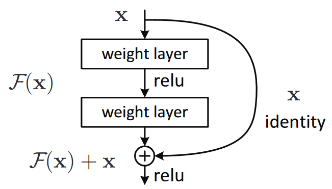
• For deep networks or if you see vanishing gradients, you can add ‘skip-connections’ parallel to the main trainable block of layers, to build residual neural networks. It allows gradients to flow from the loss down to the input and addresses vanishing gradients.

• Log every intermediate results shapes and invoke the forward pass on a small batch of random samples to make sure shapes are correct. Because of broadcasting rules, you can have silent errors when evaluating operations on tensors with the wrong shapes. Some causes of incorrect shapes can be: wrong dimension in reduce operations (sum, mean, …) or softmax, wrong dimensions in transpose/permute operations, forgetting to unsqueeze/squeeze.

Utility methods

• Fix random seeds to make sure running the same code twice results in the same result, it makes debugging easier because it excludes some of the randomness from the picture.

# for pytorch
def set_seed(seed: int):
    random.seed(seed)
    os.environ["PYTHONHASHSEED"] = str(seed)
    np.random.seed(seed)
    torch.manual_seed(seed)
    torch.cuda.manual_seed(seed)
    torch.backends.cudnn.deterministic = True
    torch.backends.cudnn.benchmark = False

# for tensorflow
def set_seed(seed: int):
    random.seed(seed)
    os.environ["PYTHONHASHSEED"] = str(seed)
    np.random.seed(seed)
    tf.random.set_seed(seed)
    tf.config.experimental.enable_op_determinism()

• It is useful to have a fully flexible implementation of the model and the data loader such that you can easily change the number of hidden layers, their dimensions, the batch size, the learning rate, etc… In particular, implementing the model, data loader and training configurations as a Dataclass makes it easy to change the parameters in only one place.

@dataclass
class ModelConfig:
    num_hidden: int
    dim_hidden: int
    dropout: float

@dataclass
class TrainingConfig:
    batch_size: int
    num_workers: int
    learning_rate: float
    weight_decay: float
    max_epoch: int

model_cfg = ModelConfig(4, 128, 0.2)
train_cfg = TrainingConfig(1024, 8, 1e-3, 1e-6, 1000)

Training

Start small

• Start with a small training and validation dataset to allow for faster iterations. Only start training on the full dataset when you are confident the model training is stable and behave as expected. In some cases, it’s also good practice to gradually increase the scale of the pipeline (more data or larger model). You don’t want to get an error after training a model for hours.

• Avoid using methods that are not necessary for a basic training (for instance LR scheduling, quantization, data augmentations, etc…) in order to reduce the size of the search space of potential bugs.

• Overfit the model on a single batch: with a large enough capacity the model should converge to the global minimum loss (e.g zero). If it does it indicates that the model is able to extract useful information. If the loss doesn’t decrease towards zero quickly, your loss might be ill-defined (like a flipped sign), learning rate might be too high, you might have numerical instabilities (like exponentiating large values), inputs and labels not aligned or a bug in the model’s implementation.

Check the loss

• Check that the initial loss makes sense: for instance if the cross-entropy loss is used, the initial loss should be close to $-\log(\frac{1}{\text{num classes}})$ if the model’s weights are initialized correctly.

\[\begin{split} \text{CE}(y, \hat{y}) & = - \sum_{c \in \mathcal{C}} y_c \log (\hat{y}_c) \\ & = - \sum_{c \in \mathcal{C}} y_c \log (\frac{1}{\text{num classes}}) \\ & = - \log(\frac{1}{\text{num classes}}) \end{split}\]

• Include some prior knowledge in the initialization: in a regression task, if you know the mean of the target is around some value $\mu$, you should initialize the bias of the last layer to $\mu$. If it is a classification task and you know you have a 100:1 class imbalance, set the bias of the logits such that the initial output probability is 0.1. It will help the training converge faster.

• Fit a simple, low capacity model to a small dataset with real data, then increase the model’s capacity (by increasing the number of layers for example). The loss should decrease, if not then there is probably a bug somewhere.

Check the convergence

• Plot loss curves as it allows to get a quick glance of the learning dynamics: does the model properly converge? Do you see large spikes? Are you overfitting at some point? Is the validation loss close to the training loss?

• Be careful when choosing the learning rate and the batch size as the two are coupled and can have a significant impact on the training convergence. The rule of thumb is to increase the learning rate by the square root of a batch size increase. Empirical studies [1] [2] show that the relation is more or less linear when using SGD and varies with the square root of the batch size when using adaptive optimizers like Adam.

• Fit the model on a set of samples with constant values (such as tensors of zeros). This data-independent model should perform worse than the one fitted on the real data and if it does, it’ll indicate that the model is able to extract useful information for the learning task.

• Log the predictions of a small validation batch during training to understand their dynamics. They should become more and more stable (that is, not that different from one epoch to another) if the model is learning correctly and in a stable way. It also helps understand if the learning rate order of magnitude is good: a small learning rate will make the predictions dynamics change slowly without an apparent lower bound while a large learning rate will make the predictions oscillate with a large amplitude during the training.

• Low convergence can be caused by “dead neurons” where gradients stop flowing back on some activations. It can happen with ReLu, and a solution is to try using a leaky ReLu or any other function that has a non-zero derivative for x < 0. You can diagnose that by checking if the gradients are zeros for a given neuron or if neuron’s inputs are negative.

• Log gradients to understand the dependencies between model’s weights. For instance let’s say you introduced a bug where information is mixed batch-wise (mixing information from different samples by using a reshape operation instead of a transpose for example). By defining a simple loss like the sum of outputs for a fixed sample and logging gradients of the input with respect to the loss, you will see non-zero gradients elsewhere than the input used in the loss, indicating that there is some unexpected dependencies between inputs. (note that you need to remove layers that do some batch-wise normalization with trainable weights as it introduces dependencies between samples but it is not a bug):

For pytorch:

# random input tensor for which we want to calculate the gradients during the backpropagation
x = torch.rand((64, 128), requires_grad=True)

logits = model(x)

# define a simple loss function that depends on only one sample
loss = logits[0].sum()

# backpropagate and calculate gradients
loss.backward()

# they sould be zero for every index != 0 and not zero otherwise
assert((x.grad[1:] == 0.0).all() and (x.grad[0] != 0.0).any())

For tensorflow:

x = tf.Variable(tf.random.uniform((16, 64)))
model = tf.keras.Sequential([
    tf.keras.layers.Dense(32, activation="relu"),
    tf.keras.layers.Dense(1)
])

# compute gradients of the input w.r.t loss
with tf.GradientTape() as tape:
    logits = model(x)
    loss = tf.reduce_sum(logits[0])

grad = tape.gradient(loss, x)

# they sould be zero for every index != 0 and not zero otherwise
assert(tf.reduce_all(grad[1:] == 0.0) & tf.reduce_any(grad[0] != 0.0))

• Logging gradient norms at different places can help diagnose very large/infinite values caused by overflows due to exploding gradients. Even without overflow, plotting gradient norms of the different layers will help detect and fix unstable training before it actually diverges if you see gradient norm spikes. In that case weight decay can help as it will add a constraint on the weight’s magnitude.

• Gradient’s magnitude relative to weights magnitude can also informs you about the training dynamics. If the gradient norm is a lot smaller than the weights norm, you have a slow training and potentially vanishing gradient issue. On the other hand if the gradient norm is much larger than the weights norm, training is instable and you have an exploding gradient issue. Of course the gradient norm should decrease during training, indicating convergence.

• Probing weight norms is also a good way to detect unstable training: a seemingly weight norm that keeps increasing can be an early sign of divergent training. Just like the point above, adding or increasing weight decay will probably help.

# for pytorch
# compute weights and their gradients norm during a forward-backward pass
names, param_norms, grad_norms = [], [], []
for name, param in in model.named_parameters():
    if param.requires_grad and "bias" not in name:
        names.append(name)
        param_norms.append(param.detach().cpu().norm())
        grad_norms.append(param.grad.detach().cpu().norm())

# plot
fig, axes = plt.subplots(nrows=2, sharex=True, figsize=(20, 20))
axes[0].bar(x=names, height=param_norms)
axes[0].set_ylabel("weight norm")

axes[1].bar(x=names, height=grad_norms)
axes[1].set_ylabel("gradient norm")
axes[1].tick_params(axis="x", labelrotation=90)

• Logging intermediate values will help detect numerical instabilities. Those can happen when using functions that can easily under/overflow, such as log or exponential functions.

• You can decompose the error as: $\text{total error} = \text{irreducible error} + \text{training error (bias)} + \text{validation error (variance)} + \text{validation overfitting}$. Model capacity/complexity addresses the bias, regularizing the variance. But sometimes (not necessarily true for deep learning models), increasing the regularization can degrade the training error. When experimenting, it is a good practice to log the contributions of each error mode across experiments to better determine where to act.

Improving the baseline

Once you have a model that trains well, you can start working towards improving the baseline performance. It can be simplified to a two steps process: increase the model capacity to decrease the loss until the model overfits, then introduce regularization to trade some of the training loss in favor of validation loss.

• The easiest regularization that doesn’t involve changing the training process nor the model architecture is to simply get more data to build a larger training dataset. It effectively allows to increase the performance of a well designed model without much risk.

• Add dropout layers.

• Add and play around with the weight decay strength.

• Add early stopping to stop the training when the model starts to overfit the training dataset (that requires a good validation dataset).

• Introduce learning rate schedulers.

• Reduce input dimensionality to either remove strongly correlated features or features that are not that informative or add too much detail/noise. It will reduce the model size allowing to train on more data with the same budget.

• Then to optimize the training procedure, you can profile the training loop in order to ensure you properly use your hardware: you can use the command watch -n1 nvidia-smi to continuously monitor GPU usage. If GPU utilization is low, it is most likely because the data loading process is the bottleneck: it takes too long, is not parallelized or there is no prefetching while the GPU is busy. In addition, you can use tools like Tensorboard to dive deeper in what’s going on during the training and identify the bottlenecks.